Jupyter notebook example

This toolbox contains functions related to the processing and generation of of wave signals.

Before this notebook can be used, the required packages should be imported.

# import default modules
import os
import sys

import matplotlib.pyplot as plt
import numpy as np

# method to import tools
try:
    import deltares_wave_toolbox as dwt
except ImportError:
    print('**no deltares_wave_toolbox installation found in environment. Path to tools manually added')
    sys.path.insert(1, os.path.join(os.getcwd(),'..','..'))
    import deltares_wave_toolbox as dwt

**no deltares_wave_toolbox installation found in environment. Path to tools manually added

How to use the spectrum class

The wave toolbox contains a spectrum class. This spectrum class can be created based on a frequency array and energy density array.

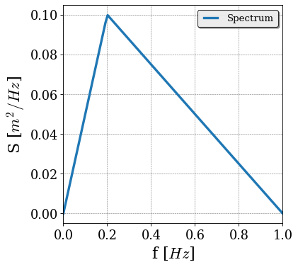
In this example, a triangular-shaped spectrum is constructed.

fp = 0.2

f_input = [0, fp, 1]
S_input = [0, 0.1, 0]

f = np.linspace(0,1,100)
S = np.zeros_like(f)

S = np.interp(f, f_input, S_input)

spec_block = dwt.Spectrum(f, S)

To plot the spectrum the function plot can be used,

spec_block.plot(xlim=[0, 1])

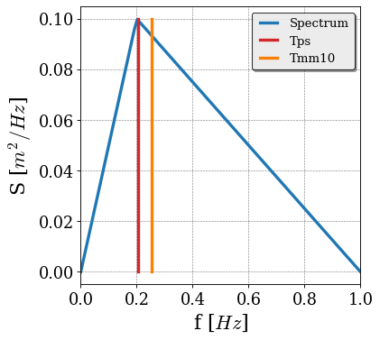
Next to plotting, the spectral properties can be computed. After the spectral properties are computed, their values are available in the class. This means that it is also possible to show the frequencies of the various computed periods in the figure of the wave spectrum.

Hm0 = spec_block.get_Hm0()
Tps = spec_block.get_Tps()
Tmm10 = spec_block.get_Tmm10()

print('Wave height:{0:.2f} m'.format(spec_block.Hm0))
print('Peak period:{0:.2f} s'.format(spec_block.Tps))
print('Spectral period:{0:.2f} s'.format(spec_block.Tmm10))

spec_block.plot(xlim=[0, 1])

Wave height:0.89 m
Peak period:4.89 s
Spectral period:3.92 s

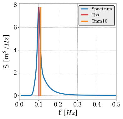
Construct JONSWAP spectrum

Besides Spectrum class, it is also possible to create a JONSWAP spectrum with the create_spectrum_jonswap function. The input of this functions is the frequency axis, peak frequency, the wave height and peak enhancement factor.

ff = np.linspace(0.01, 2, 1000)

spec = dwt.core_wavefunctions.create_spectrum_object_jonswap(f=ff, fp=0.1, hm0=2, gammaPeak =3.3)

Hm0 = spec.get_Hm0()
Tps = spec.get_Tps()
Tmm10 = spec.get_Tmm10()

spec.plot(xlim=[0, 0.5])

Low and high frequency wave parameters can also be calculated, and are saved as an attribute within the Spectrum class object.

spec.get_Hm0_HF()
spec.get_Tmm10_HF()
spec.get_Hm0_LF()
spec.get_Tmm10_LF()

print(f"Hm0_HF = {spec.Hm0_HF:.3} m")
print(f"Hm0_LF = {spec.Hm0_LF:.3} m")
print(f"Tmm10_HF = {spec.Tmm10_HF:.3} s")
print(f"Tmm10_LF = {spec.Tmm10_LF:.3} s")

Hm0_HF = 2.0 m
Hm0_LF = 7.16e-05 m
Tmm10_HF = 9.03 s
Tmm10_LF = 20.2 s

d:\checkouts\git\wave-toolbox\docs\source\..\..\deltares_wave_toolbox\spectrum.py:127: UserWarning: Cutoff frequency fmin not set, using default value of 0.45 / Tmm10
  warnings.warn(
d:\checkouts\git\wave-toolbox\docs\source\..\..\deltares_wave_toolbox\spectrum.py:277: UserWarning: Cutoff frequency fmin not set, using default value of 0.45 / Tmm10
  warnings.warn(
d:\checkouts\git\wave-toolbox\docs\source\..\..\deltares_wave_toolbox\spectrum.py:163: UserWarning: Cutoff frequency fmax not set, using default value of 0.45 / Tmm10
  warnings.warn(
d:\checkouts\git\wave-toolbox\docs\source\..\..\deltares_wave_toolbox\spectrum.py:313: UserWarning: Cutoff frequency fmax not set, using default value of 0.45 / Tmm10
  warnings.warn(

Several different wave steepness metrics are implemented as well, and are also saved as an attribute within the Spectrum class

spec.get_s0p()
spec.get_smm10()
spec.get_smm10_HF()

print(f"s0p = {spec.s0p:.2%}")
print(f"smm10 = {spec.smm10:.2%}")
print(f"smm10_HF = {spec.smm10_HF:.2%}")

s0p = 1.29%
smm10 = 1.57%
smm10_HF = 1.57%

Based on the Spectrum class a time series can be generated. The Spectrum class contains a function create_series to create a timeseries class based on a spectrum. This function assumes that the time series can be created with random phases for the individual waves. The function create_series has the start and end time of the timeseries as input together with the timestep.

timeseries = spec.create_series(10, 3600, 0.1)

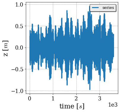
Time series class

Similar to the Spectrum class the Timeseries class also contains a plot function. When the optionaly parameter plot_crossing is set to True, all the crossings with zero are shown as well.

timeseries.plot(plot_crossing=True)

The class also contains some default signal parameters, like mean, variance, maximum and minimum:

print('variance:', timeseries.var())
print('max:', timeseries.max())
print('min:', timeseries.min())
print('mean:', timeseries.mean())

variance: 0.24998649931725056
max: 1.5631404091264942
min: -1.8211262930455447
mean: 1.819241171592356e-05

The time series class contains also functions related to individual waves. These parameters are based on the individual waves determined with a zero-crossing analysis.

For example, the \(H_{rms}\) is available. By theory the \(H_{rms}\) times the square-root of 2 is equal to the significant wave height.

Hrms = timeseries.get_Hrms()


print('Hm0: {0:.2f}'.format(spec.get_Hm0()))
print('Hrms x sqrt(2): {0:.2f}'.format(Hrms*np.sqrt(2)))

Hm0: 2.00
Hrms x sqrt(2): 1.91

But also information about the exceedance distribution is available, for example the exceedance wave height or the mean of the highest part of the exceedance distribution.

This means that we have the third definition of the (significant) wave height.

h2perc = timeseries.get_exceedance_waveheight(2)
h10perc = timeseries.get_exceedance_waveheight(10)
Hs, Ts = timeseries.highest_waves(0.33333)

print('Hm0: {0:.2f}'.format(spec.get_Hm0()))
print('Hrms x sqrt(2): {0:.2f}'.format(Hrms*np.sqrt(2)))
print('Hs: {0:.2f}'.format(Hs))

Hm0: 2.00
Hrms x sqrt(2): 1.91
Hs: 1.94

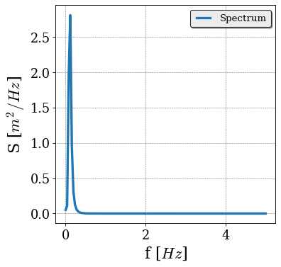
The time series class also contains a get_spectrum function to create a spectrum based on the time series.

spec2 = timeseries.get_spectrum()
spec2.plot()

To compute a bandpass filtered signal, one can use the get_bandpassfilter function:

filtered_series = timeseries.get_bandpassfilter(fmin=0,fmax=0.1)

filtered_series.plot()

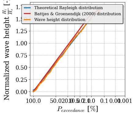
Exceedance distributions

The exceedance distribution of the time series can be visualized in three different ways:

• Histogram

• Exceedance plot

• Exceedance plot on a Rayleigh scale (this option also has the possibility to show the Raleigh and Battjes-Groenendijk distributions).

When plotting the Battjes-Groenendijk distribution, the wave height is required as input parameter. Since the timeseries object does not contain a wave height, the wave height from the spectral object is used as input.

timeseries.plot_hist_waveheight()
timeseries.plot_exceedance_waveheight()
timeseries.plot_exceedance_waveheight_Rayleigh(
    normalize=True, plot_BG=True, water_depth=8, cota_slope=250, hm0 = spec.Hm0
)

Fourier analysis

The timeseries can be transformed to Fourier components with the function get_fourier_comp.

f, xFreq, isOdd = timeseries.get_fourier_comp()

plt.figure()
plt.plot(f, xFreq)

c:\Users\bieman\AppData\Local\miniforge3\envs\dwtdev\Lib\site-packages\matplotlib\cbook.py:1762: ComplexWarning: Casting complex values to real discards the imaginary part
  return math.isfinite(val)
c:\Users\bieman\AppData\Local\miniforge3\envs\dwtdev\Lib\site-packages\matplotlib\cbook.py:1398: ComplexWarning: Casting complex values to real discards the imaginary part
  return np.asarray(x, float)

[<matplotlib.lines.Line2D at 0x1eac77aacd0>]

These Fourier components can be used to construct a spectrum with the compute_spectrum_freq_serie functions,

[f, S] = dwt.core_spectral.compute_spectrum_freq_series(f, xFreq, timeseries.nt, 0.01)

plt.figure()
plt.plot(f,S)

[<matplotlib.lines.Line2D at 0x1eac7a13010>]

Dispersion relation

One of the functions in the toolbox is the dispersion relation. In the example below, the dispersion relation is used to compute the wave celerity as function of the water depth.

depth = 20
f = np.linspace(0.001, 0.5, 100)


k = dwt.cores.core_dispersion.disper(f * 2 * np.pi, depth)



c_deep = 9.81/(2*np.pi*f)
c_shallow = np.sqrt(9.81*depth)

plt.figure()
plt.plot(k * depth, 2*np.pi*f/k/c_shallow)
plt.plot(k * depth, np.ones_like(k) * c_deep/c_shallow,'--')
plt.plot(k * depth, np.ones_like(k) ,'--')
plt.xlabel('$kh$')
plt.ylim([0, 1.5])
plt.ylabel('$c/\sqrt{g h}$')
plt.legend(['c','c deep','c shallow'])

<matplotlib.legend.Legend at 0x1eac7a52a50>

Wave decomposition

Below is an example of linear wave decomposition (i.e. seperation of incoming and reflected waves) based on the method of Zelt & Skjelbreia (1992).

t = np.linspace(0, 1800, 25000)
x = np.array([0, 0.4, 0.6, 1.2, 1.4])

## peak period
fp = [0.6, 0.7, 1.6]
## amplitudes
A = [0.1, 0.05, 0.05]
## reflection coef.
R = 0.7
## water depth
h = 0.6
## create series
zs = np.zeros((len(t), len(x)))
zs_in = np.zeros((len(t), len(x)))
zs_re = np.zeros((len(t), len(x)))
for ii in range(len(x)):
    for kk in range(len(fp)):
        k = dwt.cores.core_dispersion.disper(2 * np.pi * fp[kk], h, g=9.81)
        zs[:, ii] = (
            zs[:, ii]
            + A[kk] * np.cos(2 * np.pi * fp[kk] * t - k * x[ii])
            + R * A[kk] * np.cos(2 * np.pi * fp[kk] * t + k * x[ii])
        )
        zs_in[:, ii] = zs_in[:, ii] + A[kk] * np.cos(2 * np.pi * fp[kk] * t - k * x[ii])
        zs_re[:, ii] = zs_re[:, ii] + R * A[kk] * np.cos(
            2 * np.pi * fp[kk] * t + k * x[ii]
        )

WHM01 = dwt.Series(t, zs[:, 0])
WHM02 = dwt.Series(t, zs[:, 1])
WHM03 = dwt.Series(t, zs[:, 2])
WHM04 = dwt.Series(t, zs[:, 3])
WHM05 = dwt.Series(t, zs[:, 4])

xTimeIn_lin, xTimeRe_lin = dwt.cores.core_wave_decomposition.decompose_linear_ZS_series(
    [WHM01, WHM02, WHM03, WHM04, WHM05], h, x, np.ones_like(x), detLim=0.125
)

plt.figure()
plt.subplot(2, 1, 1)
plt.plot(t, zs_in[:, 0])
plt.plot(t, xTimeIn_lin.xTime, "--")
plt.plot(t, xTimeIn_lin.xTime - zs_in[:, 0], "-")
plt.legend(["theory", "ZS", "error"])
plt.xlim([30, 60])
plt.title("In")
plt.subplot(2, 1, 2)
plt.plot(t, zs_re[:, 0])
plt.plot(t, xTimeRe_lin.xTime, "--")
plt.plot(t, xTimeRe_lin.xTime - zs_re[:, 0], "-")
plt.legend(["theory", "ZS", "error"])
plt.xlim([30, 60])
plt.title("Re")

Text(0.5, 1.0, 'Re')